SPECIAL menu
The SPECIAL menu contains several utility routines useful in respirometry (STP conversion, altitude and pressure calculations, a metabolism estimates routine, a routine to compute ventilation) and a simple calculator.   For convenience they can be activated from the main plot window by typing specific keys, indicated by ‘key’ on the menu.

  •   SIMPLE MATH CALCULATOR...     This is an elementary math calculator (addition, subtraction, multiplication, division) with a few frequently-used functions (logs, square roots, etc.) and some specialized keys for interchanging time units (division and multiplication by 60 and 24).  If you have obtained a mean value with an ANALYZE menu operation, you can transfer that mean to the calculator for additional manipulation (note that this does not work for regression slopes).  The 'store X value...' button lets you save the result for use as a scaling factor in subsequent ANALYZE operations.  Clicking this button opens the scaling factors window.  Click on any channel's "*" or "÷" button, and the current X-value will appear in the first edit field (the multiplication or division factor) for that channel.

    • The initial X value will be set to the last computed value obtained from several of the calculators (STP, metabolism, etc.).   If no such value is available (i.e., no calculators have been used), the initial X value is set to 1.0.

    • Mathematically impossible operations (such as attempting to take the square root of a negative number) will generate a warning notice (this calculator only deals with real numbers).

    For addition, subtraction, multiplication, and division the calculator works in a simple RPN mode.  Enter the first number in the X-value edit field, hit 'return' and enter the second number, and then hit the '+', '-', '*', or '/ ' key.  Note that for performing subtraction in RPN, the ‘_’ (underline) key is substituted for the '-' (minus) key.  The result will appear in the X-value field.


  •   EXPRESSION EVALUATOR...     This routine lets you write a mathematical expression, enter numeric values for the expression variables, and have the computer solve it. The program parses the expression into components and performs the operations. The expression evaluator understands the following symbols (upper or lower case entries are OK):

    • Simple operators: + - * / ^ ( )
    • Complex operators: EXP, LOG or LN, LOG10, SIN, COS, TAN, ATN or ATAN, ABS, INT, SQR (square), SQRT (square root)
    • Two special variables (i.e., channels) named "X" and "Y", chosen with push-buttons (see image below)
    • PI (or the equivalent Greek letter)
    • Numbers (such as 5, -3.1889, and 1e-10)
    • You can add a comment at the end of your expression, delineated with the " ` " character.

    Some general considerations:

    • The 'Show instructions...' button displays the same list of permissible symbols and operations shown above. You'll need to click it again to switch off the instructions.
    • The 'Check expression' button does a preliminary parsing of the expression and indicates if there are any syntax errors (in the above example, this button has been clicked).
    • The 'Evaluate' button processes the channel data according to the expression in the upper left window. The transformed data are re-written to the main plot area. If any errors are found (see below), a warming message is shown.

    NOTE: This routine will only 'catch' errors in the basic numeric expression. It may not detect invalid or meaningless math operations that may be attempted when data are processed, such as division by zero, or taking the log or a non-integer exponent of a negative number. If such situations occur, results may be unpredicatable. The algorithm does find most such errors during processing, however.

    The underlying code for the expression evaluator was developed by the late, great Robert Purves (recently deceased and greatly missed).  I 'borrowed' it -- with his permission -- and made some modifications for LabAnalyst.  But Robert P. deserves all the credit.

    Back to top


  • STP ADJUSTMENT...   'f'  This window contains a small calculator for adjusting a measured flow rate to conditions of standard temperature and pressure (STP).  STP conversion is necessary for gas exchange calculations.  Although the gas exchange routines will perform an STP adjustment, this window's algorithm is more versatile:

    • You can select either a measure of uncorrected flow rate (in ml/min) or a cumulative volume (ml) over a measured time period (seconds).  The latter method is most useful for dry volume meters, bubble meters, etc. 
    • In addition to barometric pressure, you can account for any internal pressure within the gas flow meter (which may occur if you are using relatively high flow rates and/or small-diameter tubing).  Internal pressure can be in units of torr, PSI (pounds/square inch), KPa (Kilopascals), or mm of water (if you are using a water manometer). 
    • You can adjust the calibration temperature of your flow instrument.  Most such devices are calibrated for a temperature of zero °C, but some (like Singer dry volume meters) may be calibrated for 20 °C or other temperatures. 

    Other functions...

    • The '' button adds the current value into an internal register that is used to compute an average value (displayed with the 'show average' button).  These functions correctly account for whether the display is set for standard cubic centimeters/min (SCCM) or standard liters per minute (SLPM). 
    • The 'store flowrate' button saves the currently displayed STP flow rate as the default flow rate for gas exchange calculations (in units of SCCM).  Either an averaged flow rate or an individually-computed value are accepted, and the display setting (SCCM or SLPM) is taken into account.  In addition to saving STP flow, this button also stores a barometric pressure of 760 torr and a meter temperature of 0 °C (this is necessary to retain the accuracy of the STP conversion when computing gas exchange).

  •   ALTITUDE & PRESSURE...    'a' This option computes an estimate of mean atmospheric pressure as a function of altitude, or vice versa.  It is based on a polynomial approximation of the International Standard Atmosphere equation, obtained from the Smithsonian Meteorological Tables (as a rough approximation, pressure decreases by 50% for every 5500 meter increase in altitude).  The results should be accurate within 1-2% of actual pressure or altitude, unless weather conditions are really unusual.  Nevertheless, if you use this calculator, you need to keep a few caveats in mind:

    • Due to approximation (and rounding errors), the algorithm is not completely reversible (for example, the estimated pressure for an altitude of 2200 meters is 576.0 torr, but the estimated altitude for a pressure of 576.0 torr is 2199.7 meters).

    • The results are estimated mean values and do not account for local pressure fluctuations arising from weather changes.

    • The calculator cannot account for any pressure differential inside your system.  For example, if you use a positive-pressure ("push") respirometry system, the pressure inside the plumbing -- and hence, inside your flow meter -- will be slightly higher than atmospheric.  The opposite is true for a negative-pressure ("pull") flow arrangement.  If you want to be compulsive, you might consider using a water manometer or some other pressure gauge to measure the pressure differential and add that to atmospheric pressure during STP calculations.  In most cases, the pressure differential will be small relative to total atmospheric pressure.

    • Accuracy will decrease for altitudes above about 9000 meters (or pressures less than about 230 torr).

    • The newest versions let you use kilopascals (kPa) for pressure units, in addition to torr.

    • The 'store pressure' button will save the current value of barometric pressure.

  •       ALTITUDE SIMULATION...      This computes the concentration of an artificial gas mixture used to simulate gas concentration at a different altitude or pressure.   For example, it might be desirable to simulate the hypoxia at high altitude in a near-sea-level laboratory; this is done by using an artificial gas mixture with an oxygen concentration lower than the standard 20.95% atmospheric concentration: e.g., to simulate the oxygen partial pressure at 3,800 meters in a laboratory at sea level, one would use a gas mixture containing about 13% oxygen.
         The calculator allows estimations from different altitudes (in which case it estimates ambient pressures from a polynomial approximation of the International Standard Atmosphere equation, obtained from the Smithsonian Meteorological Tables).   It also allows estimation directly from user-entered ambient pressures -- this permits adjustments for weather or other local phenomena that shift ambient barometric pressures.

    Back to top

  •   pO2 ESTIMATION...    'o'   You can use this calculator to determine the partial pressure of oxygen (pO2) -- or any other gas species in a mixture -- from ambient temperature, ambient pressure (in the gas phase), fractional concentration of the gas species of interest in a dry gas mix, and the percent saturation of water vapor (i.e., relative humidity) in the gas phase. Oxygen (or other gases) are diluted by water vapor, and the degree of that dilution depends on RH and temperature.

    In the example at right, pressure is sea level standard atmospheric pressure(760 torr), temperature is the typical mammalian body temperature (37 °C), etc.  Note that at this temperature the saturation vapor pressure of water is about 47.6 torr (this is not affected by the total pressure in the system).

    Other considerations for this calculator:

    • The calculated pO2 value is applicable for the gas phase, and also for dissolved oxygen, as long as the solution is fully saturated with O2
    • The default pressure (torr or kilopascals, kPa) is obtained from the current data file; the default temperature is 37 °C, and the default fractional gas concentration is .2095 (20.95%, the normal oxygen content of dry atmospheric air). 

  •   DISSOLVED OXYGEN...    'w'   You can use this calculator to determine the amount of oxygen dissolved in a given volume water, as a function of partial pressure, temperature, salinity (dissolved solutes), and other factors.   Results include both the oxygen content per liter, and the total oxygen content in the specified volume of water.  Output units are user-selectable as ml O2 (STP) or mg O2.
          The default salinity value (2 parts/thousand) is reasonable for freshwater.   For seawater, use a value of 35 parts/thousand, and for typical physiological saline, use 9 parts/thousand.

    In the example at right, pressure is sea level standard atmospheric pressure (760 torr), temperature 10 °C, the water is fully saturated with oxygen, and there are 2 parts/thousand of dissolved solutes (reasonable for fairly fresh water).  The calculator provides the dissolved oxygen per unit volume, and for the total volume.

    Back to top

  •    METABOLIC ALLOMETRY...    'm'   Use this somewhat specialized utility to make estimates of an animal's resting metabolism, based on its size and taxonomic affiliation.  The metabolism calculator has many potential uses; for example, you might want to use it as a 'reality check' if you think your own metabolic data are unexpectedly high or low.
                The initial popup menu contains some very generalized equations, and also allows you to switch to submenus for specific taxa (arthropods, fish, birds, mammals, etc.).  For most taxa, several different equations are available (from different literature sources, which are described in the 'help' field to the right).  You can also pick the desired output units.  The energy equivalence of metabolism (joules per ml of oxygen consumed) can be set with the 'O2 heat equivalence' selection in the "Respirometry" submenu (EDIT menu); the default value is 20.1 joules/ml.  The mass coefficient in the allometric equation ('a' value) is adjusted to reflect whatever output unit is in use.  Results can be stored for later use.

    Metabolism for all taxa are calculated from power functions:

                metabolism = a Mb

    (where a is the mass coefficient, M is mass, and b is the mass exponent)


    This example shows an estimate of the resting metabolic rate (RMR) of a 37.3 g bird, in units of ml O2/min.  The equation was derived from a paper published by Andrew Mckechnie and Blair Wolf (the full citation would be visible if the edit field on the right was scrolled).  Note that the mass coefficient ('a' value) and mass exponent are shown and can be edited, and that mass can be in either grams or kilograms.  Also, it is possible to make corrections for the effect of body temperature by making the appropriate adjustments to the value of Tb and Q10 (in this example, the 'base' Tb, from which the equation was derived, is equal to the current Tb so no temperature correction occurs).  After changing values in the edit fields, click the 'Compute' button to display the new results.

    The 'Store' button 'remembers' the computed metabolism for later use (for example in other calculators).   The 'Save' button, if present, lets you save the current mass coefficient and mass exponent values for future use, accessed as 'Custom coefficent and exponent' option in the Taxon popup.   The 'Save' button is accessible only if the units are set to ml O2/min.   NOTE:   you will have to click the 'Save Current Preferences' button in the Preferences window if you want to have your custom values available the next time you run the program.

  •   Q10 ADJUSTMENT…     This calculates the effect of temperature (Q10) on the rate of reactions or functions -- speed, power, metabolism, etc.   To do that, enter a base temperature and an adjusted temperature, the base value of the rate function, and the Q10 (the default is 2.2), and click the 'compute adjusted value' button.   Alternately, enter the base and adjusted temperatures and the base and adjusted rate values, and compute Q10 by clicking the 'compute Q10' button.   Q10 is the factorial change in rate across a 10 °C temperature change.   The temperature difference (base temperature to adjusted temperature) can be positive or negative.

    Back to top

  •    CLOSED SYSTEM RESPIROMETRY...     This calculator computes rates of oxygen consumption (VO2) and/or carbon dioxide production (VCO2) in air or other breathable gas mixture in a closed system (i.e, the animal is sealed in an air-tight chamber for some time and metabolism is computed by the change in concentration of O2 and CO2 between initial and final gas samples).   You need to enter:
    • chamber temperature, pressure, and relative humidity (when sealed, not at the end of measurements).
    • chamber volume
    • elapsed time (between taking the initial and final gas samples)
    • initial fractional concentrations of O2 (FiO2) and CO2 (FiCO2)
    • the change in concentration (in percent) of oxygen and/or CO2, and the respiratory quotient (RQ)
          
    If you measure only one of these two gas species, the program will use RQ to estimate the other.   If you measure both O2 and CO2 concentration changes, the program will optionally use O2 in the calculation of VCO2. NOTE: it is assumed that sample gas is dried before measurement, and the default settings are:
    • Initial O2 concentration (FiO2) = .2095
    • Initial CO2 concentration (FiCO2) = .0004
    • CO2 is absorbed prior to O2 measurement
    • VCO2 is computed from VO2, if oxygen is measured, or from RQ otherwise

    Equations notes:
    • STP = standard temperature and pressure (0°C, 760 torr)
    • delta[O2] = fractional change in O2 concentration
    • delta[CO2] = fractional change in CO2 concentration
    • FeO2 = FiO2 - delta[O2]
    • FeCO2 = FiCO2 + delta[CO2]
    VO2 equations:
    • CO2 is absorbed: VO2 = STP volume * delta[O2] /(1 - FeO2)
    • CO2 NOT absorbed, compute from delta[CO2]: VO2 = STP volume * (delta[O2] - (FeO2 * delta[CO2])/(1 - FeO2)
    • CO2 NOT absorbed, compute from RQ: VO2 = STP volume * (delta[O2] /(1 - FeO2 * (1-RQ))
    VCO2 equations: NOTE: at typical delta[CO2], different equations have little effect on calculated VCO2
    • from RQ: VCO2 = STP volume * delta[CO2]/(1 - FeCO2 * (1-(1/RQ)))
    • from VO2: VCO2 = STP volume * (delta[CO2] - (FeCO2 * VO2))/(1 - FeCO2)

  •    VENTILATION...    'v'    This rather arcane calculator is for studies of ventilation (breathing dynamics) using open-flow plethysmography systems.  It will compute tidal volume (Vt, the volume of gas inspired with each breath), minute volume (Vmin, the total volume of gas inspired each minute), and oxygen extraction (EO2, the fraction of inspired oxygen that is absorbed from tidal gas).

    To support these calculations -- which are largely based on the small pressure fluctuations induced by the warming and wetting of tidal air -- you need to provide a number of variables.  Several of these are self-explanatory (at least if you know something about respiratory physiology).  Abbreviations for some of the more obscure ones are:

    • VO2, the rate of oxygen consumption
    • Tb and Ta (body and air temperature)
    • delta-P (pressure gradient between the metabolism chamber and ambient barometric pressure, in mm of water)
    • RH (relative humidity in the metabolism chamber)
    • calibration vol (the volume of gas injected during system calibrations)
    • calibration volts (mean peak height of calibration deflections)
    • calibration gain (signal amplification during calibrations)
    • sample volts (mean peak height of individual breaths in the breathing record)
    • sample gain (signal amplification when recording breathing).

    You can use the 'waveform analysis' routines in the ANALYSIS menu to obtain breathing frequeny, calibration volts, and sample volts from recorded breathing records.


    In this fairly typical example, the animal (a mouse) breathed about 6.3 times per second (not unusual for a small mammal in cold conditions) and had a tidal volume of 0.248 ml and a minute volume of about 94 ml/min.  The oxygen extraction was about 26.5%.
            Although there are a lot of data to enter, the program makes it as easy as possible.  Most values are remembered between successive uses of the calculator, so you only have to change a few edit fields (like VO2, frequency, and sample volts).  You can tab (or hit return) to move between successive edit fields.

    Back to top

  •    THERMOREGULATORY COSTS…      This specialized calculator, of interest mainly to thermal physiologists, uses weather (temperature) data from a loaded file to estimate the energy cost of thermoregulation for an endotherm:   e.g., bird or mammal.   The calculations produce a mean cost of thermoregulation, plus several related values, over whatever period the weather data encompass.

    Important caution: for temperature data, the program's default 'assumption' is that a value of zero = bad data (or no data).  If your temperatures include real values of zero, then use .001 (or some other small but non-zero number) instead of zero.

    Thermoregulatory costs are calculated using the following thermal parameters:   body temperature (Tb), lower critical temperature (LCT), thermal conductance (Cth; watts/°C), and basal metabolic rate (BMR; ml O2/min or watts; selected in the 'options' window) in a set of edit fields.   The program also asks for a channel containing time of day in hours (0-24) and two channels containing environmental temperatures (Te), one for shade and one for sun.   Note: If shade temperature is missing, the program will substitute sun temperature (if available), but only at night.   If sun temperature is missing, the program will substitute shade temperature (if available).

    For each point in the data file, the necessary metabolic rate is computed according to the following rules:

  • if the animal is day-active, whichever Te (sun or shade) is highest is used in calculations.   Note that if a day-active species never has access to sunlight (e.g., stays in deep shade), you can select the shade temperature as the sun temperature.
  • at Te >= LCT, metabolic rate is set equal to BMR (internally converted to watts)
  • at Te < LCT, metabolic rate is computed as (Tb - Te) * Cth
  • When Te < LCT in the inactive part of the daily cycle, if the animal can use torpor (selected in the 'options' window), one of two calculations are performed:

    -- if Te is at or above 1 °C less than a minimal (defended) Tb, the metabolic rate is reduced from BMR in proportion to how close Te is to minimum Tb.
    -- if Te is lower than 1°C below the minimum Tb, metabolic rate is computed as   (minimum Tb - Te) * Cth
    -- Flowcharts (decision trees) for calculations of environmental temperature and thermoregulatory costs are at the end of this section.

    Program output includes:

  • mean metabolic rate (watts)
  • factorial increase of mean metabolic rate above BMR
  • highest single metabolic rate (watts)
  • factorial increase of highest metabolic rate above BMR
  • percent of total samples for which metabolic rate = BMR (i.e., Te > LCT)
  • mean metabolic rate for all samples where Te < LCT
  • factorial increase above BMR for mean metabolic rate for all samples where Te < LCT
  • maximum daily average (watts), and expressed as factorial increase above BMR
  • maxima over 6 and 12 hours (watts), and expressed as factorial increase above BMR
  • mean metabolic rate while in torpor (watts), and expressed as factorial change from BMR
  • percent of time spent in torpor

    NOTE:   For nightime data, if a value for shade temperature is missing, the program will attempt to use the sun temperature value instead.  This substitution does not occur for daytime data.

  • These thermal calculations are performed in one of two ways:

    One individual at a time (click the 'compute costs' button):   The user enters the animal's thermal parameters in edit fields in the main program window, selects the time, sun, and shade temperature channels, and then starts calculations.  Results are shown after all Te data are processed:

           
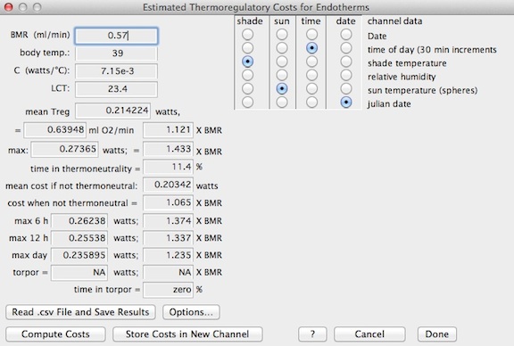
    Optionally, the computed costs for each entry in the main data file can be saved in a new channel (if the file has < 32 channels).

    Multiple individuals (species) in a spreadsheet 
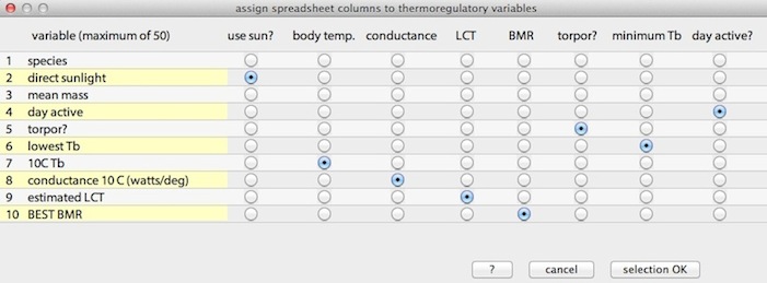
(click the 'read .csv file and save results' button):   The user selects the time and two Te channels (sun and shade) and then opens a spreadsheet file (comma separated variables; .csv) containing a series of thermal parameters for different species, sexes, etc.   The maximum number of variables in the .csv spreadsheet is 50.   Each row of the spreadsheet (up to 800) contains data for one individual or species.  You need to select the columns that contain:

  • an indicator (yes, no, y, n, 1, 0) of whether the animal can 'use' sunlight to warm itself.   If true, the calculations use the 'sunshine' value in the main data file of temperature data.
  • body temperature, in degrees C
  • minimum thermal conductance, in watts/degree C (here, degrees C is the gradient between body temperature and environmental temperature).
  • the Lower Critical Temperature (LCT) in degrees C.
  • Basal Metabolic Rate (BMR); the units are either watts or ml O2/min (selected in the 'options' window).
  • an indicator (yes, no, y, n, 1, 0) of whether the animal can use torpor to save energy during the inactive phase (night or day) of its daily cycle.
  • the minimum body temperature (Tb; degrees C) that the animal will tolerate in torpor.   The lowest environmental temperature at which this is achieved without increasing metabolism is assumed to be 1 °C lower than minimum Tb.  At lower Te, the animal will increase metabolic heat production to maintain Tb at the minimum value.   The program uses the thermal conductance value (Cth) to calculate this metabolic rate.
  • an indicator (yes, no, y, n, 1, 0, D, d, N, n) of whether the animal's active phase is during the day (diurnal) or at night (nocturnal).   A 'yes' or '1' value or equivalent means the animal is diurnal.
           
  • For each spreadsheet entry, the program runs through the Te channels from the main data file. The combined results can be saved, along with the raw data from the 'source' .csv file, in a user-selected spreadsheet file.

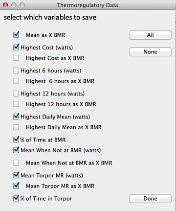
    The program always saves a column containing the mean thermoregulatory cost in watts.

    Other thermoregulatory data columns to be placed in the spreadsheet are selected from the window at right:

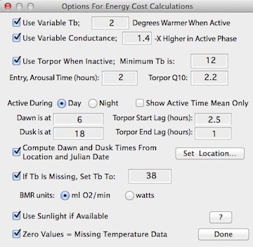
  • For both methods, the 'options' button opens a window where you can select a number of alternate ways of handling data and calculations, including:
    • the units for basal metabolic rate (BMR):   watts or ml O2/min.

    • whether to compute results for active time only (and what the hours of daylight are).   Alternately, you can get active time information from channel in a .csv data file.   Currently the hours of daylight are not obtainable from a .csv file and must be entered here.

    • whether to allow for a different euthermic body temperature during the active phase versus the inactive phase (day or night); the value in the data file (or in the main 'Thermoregulatory costs' window) is assumed to be the inactive phase body temperature.

    • whether thermal conductance also changes with the daily activity cycle (and if so, how much); the default value is a 1.4X higher conductance during the active phase.

    • a default value of body temperature if that data is missing in a .csv file entry.

    • whether to compute results assuming the animal becomes torpid during the inactive time of day (in a .csv data file this can be indicated by 'yes', 'no', or 'N' or 'n' and 'D' or 'd', or 0 and 1).

    • If torpor is used, the duration of the entry and arousal phases (body temperature is 'ramped' for calculations during these periods), the minimum defended body temperature while in torpor (this can be entered as a variable in a .csv file), and the Q10 value for adjusting metabolic rate during torpor.

    • If torpor is used, the time lags during the inactive phase for the onset and completion of torpor (which often does not occupy the entire inactive phase).

    • If torpor is used, the duration of the entry and arousal phases (body temperature is 'ramped' for calculations during these periods), the minimum defended body temperature while in torpor (this can be entered as a variable in a .csv file), and the Q10 value for adjusting metabolic rate during torpor.

      Note that if you elect to NOT allow torpor use, that restriction will apply globally to all entries in a .csv file.   If you DO allow torpor use, each entry in a .csv file will indicate whether or not torpor is applicable to that entry.

    • Whether a zero value for temperature is treated as missing data (and ignored); the alternate acceptable missing data indicator is a value of -9999.

    • Whether to use constant values for sunrise and sunset times, or compute them from location and Julian date (the day of the year from 1-365).   You will need to enter a location in latitude and longitude (fractional degrees, not degrees and minutes), and the data file with temperature information will need a veriable showing Julian date.

      Times are computed using the ‘Sunrise equation’; this example shows an annual day length cycle for a tropical latitude (~ 14 ° south).

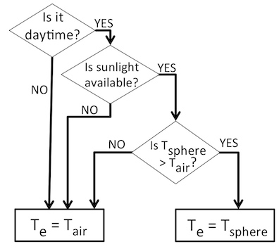
    This flowchart shows how environmental temperature (Te) is selected:

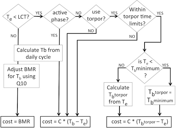
    This flowchart shows how Te, time, and physiological parameters are used to compute thermoregulatory energy costs:

    Back to top

  •    DAY OF THE YEAR...    'j'    This simple calculator will provide the Julian date (days since December 31) for a combination of date, month, and year.   It should account for leap years.

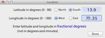
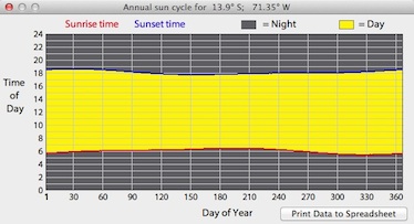
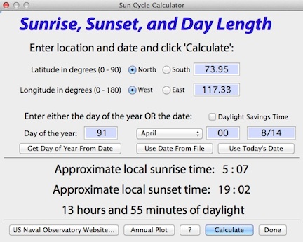
  •    SUN CYCLE CALCULATOR...     This utility uses the well-known ‘Sunrise equation’ to compute the approximate times of sunrise and sunset from date (month, day, year) and location (degrees latitude and longitude).   You need to select North or South latitude, and East or West longitude relative to the Prime Meridian.
             NOTE: The program expects latitude and longitude in fractional degrees, not degrees and minutes. Thus 27° 30’ north should be entered as ’27.5’ (i.e., halfway between 27° N and 28° N).

    Sun time estimates are approximate for several reasons:

    • Sunrise and sunset times are based on local solar noon (i.e., when the sun is at its zenith (highest above the horizon) from the perspective of the observer’s position.   This is likely to be slightly different from local time.   As defined by people, time zones are arbitrary, and since they are roughly 15 ° of longitude wide and often do not run strictly north and south, sunrise and sunset times can vary by an hour or more with a single time zone.

    • The calculator has no allowance for elevation above sea level (which makes rise times earlier and set times later, if the horizon is at sea level).   It also has no allowance for local topography — for example, if the observer is in a deep valley, the visual horizon is elevated above the ‘real’ horizon, and rise times will be later and set times will be earlier than shown here.

    • The precise times of sunrise and sunset are of concern to astronomers and the like, but for most purposes they are rather ‘fuzzy’ due to the angular diameter of the solar disc (about 32 minutes of arc or 0.53 degrees), atmospheric refraction, etc.

    NOTE: The U.S. Naval Observatory hosts a web page (USNO Sun and Moon Data) that permits very accurate calculations of solar and lunar data.  It incorporates ‘fixes’ for many of the issues described above, and — if you are connected to the internet — can be accessed with the ‘Naval Observatory Website’ button.

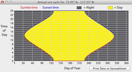
    • The 'Annual Plot' button will compute and display an entire year's day length cycle, based on latitude-longitude position.   The 'Print Data to Spreadsheet' button makes a tab-delineated .xls spreadsheet containing the annual cycle (date, sunrise time, sunset time, and day length).   This example shows a Polar-region cycle, with complete darkness in winter and 24-hour sunlight in summer:

  •    UNIT CONVERSIONS...    'u'     This provides a number of unit conversion options for distance, mass, area, pressure, temperature, rate time units, energy, water loss, light intensity.   It is similar to (but more comprehensive than) many of the options in the 'transformations' routines in the EDIT menu.   You need to select a general type of conversion from four choices, then pick the specific conversion from the pop-up menu.  For some conversion, text describing special conditions will appear.
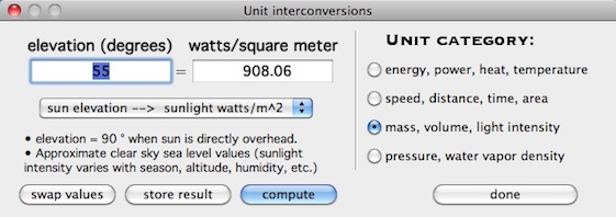
  • Back to top


    Other links: