| |
Waveform analysis
|
|
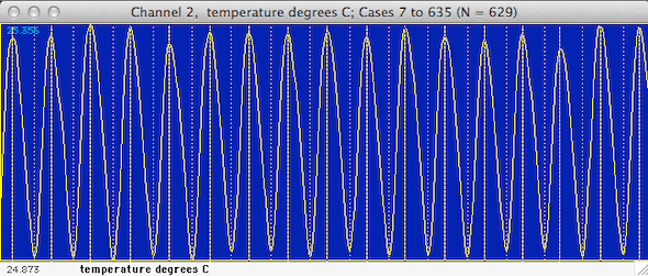
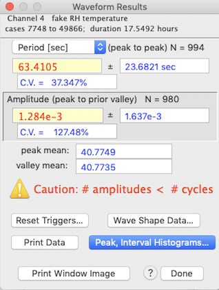
WAVEFORM... ⌘W Uses simple algorithms to calculate wave frequency and mean peak height. Basically, the program looks for successive 'peaks' and 'valleys' in the data. A peak (the 'crest' of a waveform) is defined as a series of 5 points with the middle point having the highest value, and with values declining in the two points on either side. The inverse is true for a valley (the 'trough' of a waveform). LabAnalyst marks the peaks and valleys it finds with dotted (valleys) or dashed (peaks) lines in the block window (see below). In the default mode the program will use all the data within the block. Alternately, 'filtering' is possible through cursor selection of minimum peak and valley values ('triggers') in the block window. Click the 'use cursor' button and move the cursor to the block window. A horizontal line will track the cursor's movement and a readout in the Results window will show the height of the cursor. Click once to select a peak (done first) or valley trigger. After selection, peak triggers are shown as pink lines, and valley triggers are green lines. The post-peak trigger value (default zero) is the number of cases the program 'skips' after finding a peak. This option can be useful when analyzing noisy files. A typical results window is shown at right, above. Note that in this example the number of periods and amplitudes is correctly matched. The program beeps and prints a warning if no periodicity is found, if no amplitudes are found, or if the number of amplitudes does not equal the number of cycles +1 (indicating that some peaks were not associated with definable valleys, so the frequency or amplitude may be incorrect). The mean values for both peaks and valleys are also shown. NOTE: The waveform algorithms are easily confused by noise (because of the way peaks and valleys are defined). If you are only interested in frequency, it is reasonably safe to reduce noise by smoothing data prior to analysis. However, smoothing reduces peak amplitudes (in some cases very dramatically), so it must be used with caution if you need peak height data. Smoothing is least damaging if peaks are 'rounded' and contain many more points than the smoothing interval. If necessary, use PAIRS DIFFERENCE to obtain peak heights, then obtain frequency data after smoothing. You can obtain some additional information about the waveform besides mean frequency and amplitude using the following options: 
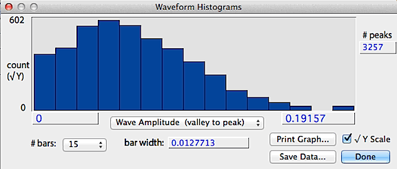
Rise time (the elapsed time from a valley to a subsequent peak) is shown in blue; decay time (the elapsed time from a peak to a subsequent valley) is shown in red. The small triangles indicate the means while the bars show the distributions. The save data button stores a text file of the histogram values, the print graph button sends the data to a printer, and the square-root Y button shows the count as a square-root, which better shows bars with low counts.
|