This describes the portion of the EDIT menu covering topics other
than respirometry. See the Respirometry
submenu for gas exchange calculations.
For BASELINE, INTEGRATE, DERIVATIVE, SMOOTHING, GAS EXCHANGE,
and some other EDIT menu calculations, clicking the plot window is
equivalent to clicking a highlighted button.
To change channels, go to the CHANNELS menu, use the up
and down arrow keys, or push the desired channel number on the keyboard
('0' for 10; for higher channel numbers push shift+number, i.e., shift-2
for channel 12).
UNDO  Z Replaces the most recently changed
channel with its previous value. This allows you to recover, without
reloading the original file from disk, if you make a mistake during a transformation
or other manipulation. Z Replaces the most recently changed
channel with its previous value. This allows you to recover, without
reloading the original file from disk, if you make a mistake during a transformation
or other manipulation.
When performing a complex sequence of manipulations
on data, remember that only one level of UNDO is available. For some operations that affect all channels, NO UNDO is possible. |
CUT
TEXT X
COPY TEXT C
PASTE TEXT V CUT, COPY, and PASTE work like the
normal Apple operations, but only on text (not on items like data
blocks.).
CLEAR BLOCK Clears
any currently selected block and closes the block window (if open).
Note: hitting the 'esc' or 'clear' key has the same
effect.
SELECT ALL DATA A Selects a block of data that includes
all of the cases in the file.
EDIT FILE DATA... E Allows editing of channel labels (within
the limit of 30 characters -- including spaces -- per label), along with
mass, barometric pressure, effective volume, etc. The edit window
looks like this:
By clicking one of the 'channel x' buttons, you can change to
the selected channel. Comments can also be edited up to the maximum
of 32K characters (240 characters if you
want to save in Sable SSCF format).
Clicking on the 'comments' window in the main display takes you directly
to the 'edit comments' window.
Back to top
CORRECT BASELINE... B (Active channel
only) There are seven methods of baseline correction. You should select
the one most appropriate for your data set.
1. Automatic -- The program selects
blocks at the start and/or end of the data and uses them in a regression
to compute the baseline. You can change the number of cases in these
blocks by editing the value in the box (the default is 15). Use the
automatic method only if the beginning and end
of the file contain nothing but true baseline values.
If this condition is not met, use another method (such as #2 or #3, below).
2. Automatic (periodic) -- (shown
at right, above) The program uses one of two methods to identify baselines:
(a) you use the cursor to select a starting point and time interval between
reference readings, and the program uses them to 'step' from reference
to reference, or (b) the program uses markers in each reference as a cue
for baseline setting (in my experience, this works considerably better than the first method). You can chose which marker is the reference indicator,
and whether the reference adjustment should begin on either side of that
marker. Only the latter method (using markers) can be scripted.
3. Use the mouse to select a sequential series
of baseline blocks (multiple points), starting
from the 'left' end of the file and moving to the 'right' end. This
method corrects the baseline in a series of segments (up to 300 in a given
file; you can repeat the process if you need to handle more than that).
Alternately, you can click on single points (instead of selecting
blocks).
4. Use the mouse to select beginning and ending
blocks, which LabAnalyst X then
uses in a linear regression to compute the baseline. Alternately,
you can click the single point button to pick baseline points (instead
of selecting blocks).
5. Use the mouse to select a single
block which the program uses to calculate a flat baseline. Alternately,
you can click on a single point (instead of selecting a block).
6. Keyboard entry of beginning and ending
baseline values.
7. Keyboard entry of a constant baseline value.
For all methods except #2 (automatic periodic references) or #3 (multiple
blocks), the baseline is drawn on-screen (if it fits within the current
Y-axis scale) and you can cancel, reselect, or select it. The final
baseline is drawn across the entire file.
See the Reference removal section
for an easy method of eliminating baseline sections for analysis.
LAG CORRECTION...
(Active channel only). Asks for the number
of seconds of lag time (for example, if the response of one channel is delayed
relative to some other channel). The channel is 'left-shifted' (time
is advanced) by the chosen amount. On the right end of the trace,
a group of samples equal to the lag interval is set to zero.
The main goal of lag correction is usually to correctly synchronize two
channels. To determine how much lag time to use, follow these steps:
- Identify a short-duration event (a sudden change) that affects both
of the channels in question.
- With either the Overlay command or the Multi-Channel
Display command (in the VIEW
menu), place both channels on the screen.
- Mark a block that extends from the event on one channel to the same
event on the other channel.
- Use the Basic Stats
option (ANALYZE menu) to determine
the time difference (the block duration can also be read at the top of
the Results window). This value should be used as the lag correction
for the delayed channel.
Back to top
INTEGRATE...
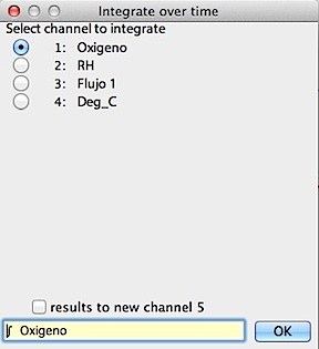 I Sequentially
adds all points from the first to the last to get a cumulative curve (this
is not 'true' mathematical integration). The window looks like the
example shown here (note that the program places an integral sign in front
of the original file label):
DERIVATIVE... D Goes from
the last point to the first point (right to left), computing and storing
the change between successive points (this is not 'true' mathematical
derivation). The derivation window is nearly identical to the one
shown at right for integration (and the program places a derivation symbol
in front of the original file label). I Sequentially
adds all points from the first to the last to get a cumulative curve (this
is not 'true' mathematical integration). The window looks like the
example shown here (note that the program places an integral sign in front
of the original file label):
DERIVATIVE... D Goes from
the last point to the first point (right to left), computing and storing
the change between successive points (this is not 'true' mathematical
derivation). The derivation window is nearly identical to the one
shown at right for integration (and the program places a derivation symbol
in front of the original file label).
- For both integration and derivation, if the number of channels is less
than 24, you can place results in a new channel.
| NOTE: Because
numbers are stored in floating point format with 8-10 digit precision, integration
may result in loss of least-significant digits, particularly if the
numbers are large (i.e., if their cumulative sum contains more than 8-10
decimal digits). Thus integration followed
by derivation of the same data will not necessarily produce a result identical
to the original data. Normally this poses no problems to
users. |
SMOOTHING... F (Active channel
only) Performs nearest-neighbor smoothing with a choice of 3, 5, 7, 9, 11,
15, 19, 25, 35, and 51- point averaging intervals with one or more smoothing
repetitions (the default is 1). The smoothing interval is the number of
adjacent cases averaged for each smoothed point. For example, 5-point smoothing
includes the data point itself, the two immediately earlier points, and
the two immediately later points in the averaged value.
 The program makes a memory copy of the channel
and uses it as its data source (this insures that within a given smoothing
iteration, previously smoothed data are not part of the calculations).
When smoothing is complete, the channel is redrawn. If a block has
been selected, you can smooth either all the data or just within the block.
You can also smooth conditionally, changing only those data within a certain
range (i.e., greater than or less than user- specified values). If
the file contains less than 24 channels, you can copy the active channel
to a new channel before smoothing. The program makes a memory copy of the channel
and uses it as its data source (this insures that within a given smoothing
iteration, previously smoothed data are not part of the calculations).
When smoothing is complete, the channel is redrawn. If a block has
been selected, you can smooth either all the data or just within the block.
You can also smooth conditionally, changing only those data within a certain
range (i.e., greater than or less than user- specified values). If
the file contains less than 24 channels, you can copy the active channel
to a new channel before smoothing.
The example at right shows 19-sample smoothing to be repeated over six
cycles. Notice that the indicated smoothing interval (calculated from
the sample interval and the averaging interval of 19 samples) is 27 seconds.
Conditional smoothing is selected, and smoothing will be applied only to
data points will values less than 0.15.
Smoothing can be repeated as often as necessary, but be very careful
that you do not obliterate useful information from the data. For example,
smoothing a high-frequency waveform may result in a substantial decrease
in the peak amplitude, although this should not affect frequency calculations.
Remember that you can undo only the last smoothing operation performed.
Back to top
REMOVE SPIKES...
(Active channel only) Allows you to remove voltage
'spikes' or other inaccurate data, either automatically or interactively.
There are several options for removing spikes:
Automatic:
Single-point spikes that exceed a user-defined amplitude are easily
removed with the spike sweep operation. However, this will
not work effectively for multiple-sample spikes. Spike sweep searches
for single data points that differ from their nearest neighbors by the threshold
value or greater (in absolute units). Points meeting these criteria
are converted to the average of the two nearest neighbors.
Two options are available for sweeping: 'Single scan' makes a
single pass through the data; 'Spike sweep' repeats scanning until
all appropriate spikes are removed.
The trim data  option searches for data points that are greater
or less than preset limits; all data outside these limits are set to user-defined
values. Both sweep and trim can be performed within
blocks only (if a block has been selected). option searches for data points that are greater
or less than preset limits; all data outside these limits are set to user-defined
values. Both sweep and trim can be performed within
blocks only (if a block has been selected).
In this example, the user has performed a spike sweep with a threshold
value of .75, and the program found and removed 5430 spikes. Also,
the trim data options have been set such than any value exceeding 5 will
be set to equal 5, and any value less than -.15 will be set to zero.
Interactive: In Spike
mode, spikes are selected by clicking on them with the crosshair cursor.
The program replaces the selected point with the average of the two values
on either side. This is most effective for spikes of short duration
(optimally, a single sample).
 An alternate noise-removal method is 'Data
Linearizing'. This mode linearizes all data points between two
selected points (as shown schematically in the example plot). Points can be selected by single clicks, or by the standard click-hold-drag method. Optionally
(as shown here), you can select the 'Interpolation markers' option
to automatically insert the standard double-arrowhead interpolation markers
at the beginning ("»") and end ("«") of
linearized intervals (this lets you avoid using interpolated data in most
analyses). An alternate noise-removal method is 'Data
Linearizing'. This mode linearizes all data points between two
selected points (as shown schematically in the example plot). Points can be selected by single clicks, or by the standard click-hold-drag method. Optionally
(as shown here), you can select the 'Interpolation markers' option
to automatically insert the standard double-arrowhead interpolation markers
at the beginning ("»") and end ("«") of
linearized intervals (this lets you avoid using interpolated data in most
analyses).
If you want to conserve the short-term variation in the data within the
'linearized' area, select the 'Conserve variation' option.
This uses a 3-point nearest-neighbor smoothing operation to reduce the amount
of deflection within the defined area, but it preserves the point-to-point
variation. You can select how much linearizing will occur with the
pop-up menu of smoothing repetitions ('smooth once' = 1 smoothing
pass, i.e., the most variance preseved, and 'smooth X5' is 5 smoothing
passes, resulting in the greatest degree of linearizing). As more
smoothing passes are added, the corrected data increasingly resemble a straight
line between the beginning and ending points (this is best visualized by
experimenting with the three options, using the 'delete' key after each
one to eliminate the correction).
You can alternate between spike removal mode and linearizing mode by
first clicking in the lower left window, then clicking the desired mode
button, and finally returning to the plot area. Accessing the 'Quit'
button is done similarly.
If you are in multi-channel display mode, the program will shift to single-channel
display (of the currently active channel) for spike removal operations.
If the file contains more than screenwidth cases and you are in Entire
File display mode, the program will shift to Active Screen mode when interactive
spike removal is selected. Use the screen slider to shift between
screenfulls of data (note that the data linearizing option can work across
screen boundaries).
REMOVE REFERENCES... (Active
channel only) Reference readings are a common method of checking measurements
against a known value. Typically one reads sample data for a certain
period, after which the instrument is switched to read some standard condition
(perhaps a known temperature or gas concentration). After the reference
reading, more sample data are recorded, and the process is repeated as necessary
(the LabHelper program can do this automatically,
for example). References help insure accuracy, but may be inconvenient
during analyses. This routine lets you eliminate most kinds of reference
readings from a channel.
The Remove references window is shown above. To use it you
need to specify:
- Whether references are 'downwards' or 'upwards'. A 'downwards'
reference -- such as in the example -- is one in which the reference data
have lower values than the sample data, and an 'upwards' reference
is one in which the reference data have higher values than sample
data.
- The reference index value. If you have specified a 'downwards'
reference, the program assumes all data with values less than the
index value are to be considered reference data (vice versa if you specified
an 'upwards' reference). In the example, the index value is set at
0.022.
You can also use the cursor to select a reference index cutoff, using the 'Set reference cutoff with cursor' button. Move the cursor until the indicated line is acceptable, and then click the mouse.
- The number of extra cases. Reference readings are seldom instantaneous
events; usually there is a gradual change -- over a fairly constant number
of samples in a particular data channel -- between 'true' sample and 'true'
reference values. This period of change needs to be excluded from
reference removal calculations. The value you specify as 'extra cases'
is the number of excluded samples on either side of points identified using
the reference index value -- in this case, five samples.
- Whether reference data are interpolated between initial and final values,
or replaced with a fixed value. In interpolation, the computer fills
in the reference gap by 'drawing' a line between the initial and final
values. This is essentially the same operation as can be done manually
using the 'linearizing mode' option in the spike removal window.
Reference removal is performed and the new values are displayed in the
plot area when you click the 'Fix references' button. You can then
undo the results, or exit the function.
RESPIROMETRY
 This selection
is a submenu. See the Respirometry
page for details.
SIMPLE TRANSFORMATIONS...
T This
option allows various mathematical manipulations such as logarithms (base e and
base 10), inverses, exponentiation, multiplication, division, square-roots,
Q10 correction, etc. Several cross-channel operations
are also possible (addition, subtraction, multiplication, division).
A polynomial conversion with one to nine degrees is available. Results
are stored in the first source channel, or optionally (if the number of
channels is less than 24) in a new channel. This selection
is a submenu. See the Respirometry
page for details.
SIMPLE TRANSFORMATIONS...
T This
option allows various mathematical manipulations such as logarithms (base e and
base 10), inverses, exponentiation, multiplication, division, square-roots,
Q10 correction, etc. Several cross-channel operations
are also possible (addition, subtraction, multiplication, division).
A polynomial conversion with one to nine degrees is available. Results
are stored in the first source channel, or optionally (if the number of
channels is less than 24) in a new channel.
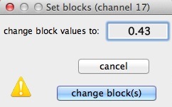
If a block is selected, a button and edit field (not shown here) will let you set all the values within the block to a fixed value (the default is zero).
This sample window shows the addition of two channels, with the result
stored in a new channel. The multiply/divide option is set to 1 (meaning
that no action is taken on the result of the addition operation).
If you set this number to something other than 1.0 and click either of the
multiply or divide buttons, the result of the 'main' operation will be adjusted
accordingly.
Two buttons at left toggle between transformations and unit conversions. The operations for transformations are selected from the
smaller (right-most) of the two pop-up menus shown at near right.
Note that the last five transformations (addition, subtraction, multiplication,
and division with different channels, and Q10 correction
from a temperature channel) are only available if the file contains more
than one channel.
Alternately, you can use a range of unit conversions from the pop-up
menu shown at near right. These pertain to commonly-used units of
energy, flow rate, pressure, mass, speed, temperature, water vapor pressure,
gas volume, and so forth. Conversion into mass-specific units is also
available. The 'STP converter' option does not affect the channel
data, but allows you to calculate an appropriate correction for temperature
and pressure effects on gas volume (useful in respirometry).
For most of these operations, the conversion factors (i.e., the numerical
coefficients in the conversion equations) can be edited as desired prior
to calculations. For example, you may wish to adjust the conversion
factor for the heat of vaporization of water (which is set for a default
evaporative surface temperature of 37 °C) to a value accurate at some
other temperature.
Many of the conversions will attempt to adjust the channel label as appropriate.
For example, if you have chosen to convert a channel to mass-specific units,
the program will append a "/g" or "/Kg" to the end of
the current label. Similarly, if you are converting a channel with
units of watts to units of KJ/day, the program will search the label for
the word "watts" and replace it with "KJ/day".
Keep in mind that automatic label modification is not always successful
(depending on the format of your channel labels), so be sure to check.
Note that the transformations routines do not make any attempt to adjust
labels to reflect changes. You should be diligent in correcting the
file labels appropriately in order to avoid confusion later on.
During mathematically complex operations that are time-consuming (such
as calculating logs or computing vapor pressure from temperature), a progress
bar appears. This isn't shown for faster operations, since drawing
the progress bar often is slower than the computations themselves!
Some special considerations for transformations
and conversions:
- If the file contains less than 24 channels, you can copy the active
channel to a new channel before transforming or converting it (this is
a convenient way to duplicate channels), or route the converted file to
a new channel.
- If a block has been selected, it can be set to a user-selectable value
(default = zero) with the 'set block' button.
- If a block has been selected, you can optionally transform the all
the data or just within the selected block.
- With many transformations, you can scale the results by multiplying
or dividing them by a user-defined constant (select the 'multiply' or 'divide'
button, as described above).
- The 'STP converter' option in the conversions menu is a small
calculator that computes the flow rate at Standard Temperature and
Pressure (STP) from the prevailing conditions of temperature, pressure,
and flow. It does not modify any channel data.
The response correction option is similar to the 'effective volume'
computation used for gas exchange. It compensates for capacitance-like
characteristics that slow response times and obscure rapid changes in measured
variables, using the "Z-transformation". The algorithm compares
successive values and corrects them according to the following equation:
corrected value = [(value-last value)/Z
factor] + last value
Typical Z factors are between 0.1 and 1.0 (other values are accepted).
It is reasonable to determine the correct value by trial-and-error, if you
have a recording that contains a known step change (or near-instantaneous
change). Apply different Z factors until the results approximate a
step change.
The breakpoint transforms option lets you use different transformation
equations depending on whether data are less than or greater than a user-specified
'breakpoint' value. You enter the equations and the breakpoint in the following
window (which appears whenever you select the breakpoint option):
After entering the breakpoint value, pick the type of equation for data
below the breakpoint value, using the radio buttons at left. Then
click the 'use this equation for data < breakpoint' button, and
enter the a, b, and c values in the first set of edit fields at the bottom
of the window. Then select the equation type for data equal to or greater
than breakpoint, click the 'use this equation for data > breakpoint'
button, and enter the a, b, and c values in the second set of edit fields.
In this example, a 2-way polynomial will be applied to data < breakpoint,
and an exponential equation will be applied to data > breakpoint. When
all is correct, click the 'OK to transform' button to return to the main
Transformations and Conversions window.
- If the screen width is sufficient, a scrolling edit field with instructions
appears at the right of the window
- For all equation types, initial values always leave the data unchanged
(i.e., they multiply by 1.0).
| NOTE: LabAnalyst
X does not allow invalid or meaningless mathematical operations,
such as division by zero, taking the log of a negative number, or using
a non-integer exponent on a negative number. If LabAnalyst
X encounters these situations during a transformation, the offending
cases are set to zero, the computer beeps, and a warning message appears.
At this point you can click the 'Cancel' button to discard the transformed
data, or accept the (partially invalid) transformation. |
For related operations, see also the SCALE
RESULTS option (ANALYZE menu).
EXPRESSION
TRANSFORMS... This routine lets you write a mathematical expression
to transform a channel. The program parses the expression into components
and performs the operations. The expression evaluator understands
the following symbols (upper or lower case entries are OK):
- Simple operators: + - * / ^ ( )
- Complex operators: EXP, LOG or
LN, LOG10, SIN, COS, TAN, ATN or ATAN, ABS, INT, SQR (square), SQRT (square
root)
- Two special variables (i.e., channels) named "X" and
"Y", chosen with push-buttons (see image below)
- PI (or the equivalent Greek letter)
- Numbers (such as 5, -3.1889, and
1e-10)
- If you wish you can add a comment at the end of your expression, delineated
with the " ` " character.
Results are stored in the first of the source channels, or optionally
(if the number of channels is less than 24) in a new channel (edit the file
label as appropriate). If a data block has been selected, you can transform
all the data or just within the block. A typical expression transforms
window looks like this:
Some general considerations:
- The 'Show instructions...' button displays the same list of
permitted symbols and operations shown above. You'll need to click it
again to switch off the instructions.
- The 'Check expression' button does a preliminary parsing of
the expression and indicates if there are any syntax errors (in the above
example, this button has been clicked).
- The 'Run transform' button processes the channel data according
to the expression in the upper left window. The transformed data are re-written
to the main plot area. If any errors are found (see below), a warming message
is shown.
- The 'undo' button reverses the effects of the last transformation.
- If a data block has been selected, you can transform all the data or
just within the block.
NOTE: This will only 'catch' errors
in the basic numeric expression. It may not
detect invalid or meaningless math operations that may be attempted
when channel data are processed, such as division by zero, or taking
the log or a non-integer exponent of a negative number. If such situations
occur, results may be unpredicatable. The algorithm does find most such
errors during processing, however.
| The underlying code for the expression evaluator
was largely developed by Robert
Purves (recently deceased and greatly missed). I borrowed it -- with his permission -- and
made some modifications for LabAnalyst X.
But Robert P. deserves all the credit. |
SCALE TO BLOCK...
Resets the scale and range of the data to values specified by the user,
based on a block of data. For example, you can rescale a block of data with
an initial range of -.134 to .335 to a new range of zero to 100% (or any
other upper and lower limits).
Note: although calculations are based
on data within the selected block, the scale and range adjustment is applied
to the entire file.
If you use the 'Block only' option, the rescaling is applied only
to the selected block -- but keep in mind that it will now be out of calibration
with the rest of the data in the channel.
BLOCK SCALE, 0-100%
This option automatically scales the selected block to a range of zero
to 100.
Back to top
COMPACT & AVERAGE...
Makes a compact version of the data by breaking
it into a series of blocks of user-specified length, and then computing
a mean and S.D. for each of the blocks. Each block contains
a fixed number of cases, and the block duration (in time units) depends
on this number and the sample interval.
Compacted data can be saved as tab-delineated
text files containing both means and standard deviations. It is also
shown on-screen in the regular plot area. This can make it easier
to see trends in noisy data, and is also useful for preparing data for publication
-- a figure broken into a series of means and S.D.s is frequently easier
to read than a simple line plot (particularly if the raw data are somewhat
noisy).
NOTE: although the plot area on the screen shows the compacted
version, any analyses are performed on the original data, which is shown
as normal in the block window.
This example shows a 20-fold compaction, which equates to a 'block size'
of 30 seconds for each mean and S.D. computation. The 'highlight
data means' and 'show S.D.' options are selected; this will show the mean
values as a dot, and the SDs as vertical lines in the plot area (in active
screen mode only if there are more than screenwidth
cases).
Some operations, like Baseline with user-selected points, are
difficult to use if the data are shown in compacted form (although you can
still read the uncompacted values for the cursor position in the data bar).
It's probably best to shift to the regular display ('normal plot') for these
operations.
CHANGE OR REMOVE This selection is a submenu with three items:
CHANGE BLOCK
This option allows you to replace the values
within a selected block with a user-defined constant. Optionally,
you can do this to multiple blocks simultaneously. This is useful
in many situations. One example is if you wish to apply the 'minimum
value' analysis operation, but your data contains some reference readings.
By marking the references and then changing them to some arbitrary large
value, you can scan the complete data set and the analysis will be restricted
to 'real' data instead of being confused by reference points.

REMOVE BLOCK
This option removes the data within a marked
block, either within a single channel or for all the channels (the 'entire
file' option). In either case, the elapsed
time and time-of-day readouts in the data bar are no longer accurate
for data points later in the file than the removed segment. The one exception to this rule is if you deleted a block at the beginning of the file (i.e., starting at the first case).
- If you apply this operation to a single channel of a multi-channel
file, any markers are not adjusted, and therefore are no longer accurate
for the adjusted channel (they are OK for the other channels). Also,
data in the adjusted channel are no longer correctly synchronized with
data in the other channels. It is possible to 'undo' a block cut
from a single channel.
- If you cut a block from the entire file, any markers are adjusted so
that they are correctly synchronized with the data, and data in all the
channels remains synchronized. The 'undo' option does not work if
a block is cut from the entire file.
REMOVE CHANNEL K This option removes one or more entire
channels from the file. At least one channel must remain. The
'undo' option cannot restore a channel or channels after they are removed
from the file.
CROP FILE TO BLOCK...
If you have a selected block, this option will delete all of the cases outside of the block (like 'cropping' a photograph). The crop is applied to all channels, and cannot be 'undone' (however, it does warn you of this risk). After the crop, the time indicators remain accurate but in some circumstances (drastic crops of long-duration files) the date indication may be incorrect (you might lose a day; this can be fixed in the EDIT FILE DATA option).
DUPLICATE CHANNEL
Makes an identical copy of the currently active channel, and makes the
new copy the active channel (this only works if the number of channels is
less than 24).
RE-ARRANGE CHANNELS This window lets you shift the order of the channels in a file (it also allows channel duplication and channel deletion). The window shows the current channel order; you click channel-indicator buttons ('next...') in the order you desire the new arrangement to be. This image shows channel order selection in progress, with three channels chosen out of six:

A check-button lets you opt to have a suffix indicating re-arrangement appended to the file name.
NOTE: This operation is not undo-able.
RECORD EDITS
This option (on by default) records every action that changes a file's data in the file's comments, so they can be reviewed later.
FIX ENDIAN BYTE ORDER
PowerPC and Intel processors store numeric data in different formats (most significant bit first or last). If you try to read data obtained on a PPC on an Intel machine, the information will be wildly incorrect. LabAnalyst usually finds and fixes any such problems transparently, but this option lets you perform the conversion manually.
Back to top
|