OPEN WARTHOG...  O Loads data files produced by LabHelper
or LabAnalyst X. There are four types: O Loads data files produced by LabHelper
or LabAnalyst X. There are four types:
 Warthog-format
text files Warthog-format
text files
(chart or oscilloscope)
|
 raw binary chart data
|
 raw binary scope
data
raw binary scope
data
|
|

| binary edited data (saved from LabAnalyst) |
|
The file opening box highlights only these types. Two are binary formats, for LabHelper
and edited LabAnalyst X files: the older
Binary-Coded Decimal (BCD) and Floating-Point (FP). LabAnalyst
X will transparently read either, but will write only in
FP format. The main difference is speed: BCD
files load fairly slowly (since they are read and converted one sample
at a time), while FP files load quickly (since entire channels
are read directly from disk into memory).
 If you click the toolbar 'Open' or 'Append'
buttons, you will get this window if you've not specified
in the 'Preferences' window that
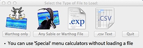
only Warthog files will be shown: If you click the toolbar 'Open' or 'Append'
buttons, you will get this window if you've not specified
in the 'Preferences' window that
only Warthog files will be shown:
This gives you the choice of Warthog (current or 'classic' files obtained prior to OS X), ASCII (text) or Sable SSCF or ExpeData files
(see below).
Note: If you select Sable files, you can also load Warthog-format files (the program checks the file type and loads whichever is correct) -- but if you attempt to load a file that isn't Warthog or Sable format, you'll get an error message.
IMPORT
 This
submenu has three items: This
submenu has three items:
WARTHOG-FORMAT TEXT FILE... For data
files of any type -- as long as they are in Warthog binary format
or Warthog text format. WARNING: only files with these formats will load properly.
WARTHOG BINARY FROM 'CLASSIC' OS9... For old
Warthog binary files from prior to OS X. WARNING: only files with these formats will load properly.
TEXT FILE... Loads text (ASCII) spreadsheet files with
variables delimited by commas or tabs (spaces do not work as delimiters).
The first few cases are shown, including
symbols for delimiters. You can specify where to start reading data
(to avoid non-numeric text headers, etc.), and elect to ignore selected
variables in the 'list'; some of which (as in the example below) don't
contain useful data. You need to specify the correct sample interval (in seconds).
The program will automatically read all of the data up to the
maximum size. After loading, you can enter appropriate variable names, start time, start date, and comments. The text file import window
looks like this:
This example contains 6 variables (only 5 of which are used; the fifth
is ignored). Data input will begin at
line 3, line 1 will be used as variable names, and the
user has specified a sample interval of 5 seconds.
• Note: current versions show a slightly different window with a horizontal grow tab at lower right.
SABLE
FILE... Loads Sable
Systems data files in SSCF format or the similar but newer 'ExpeData' format. Nearly all Sable files will load;
those which have more than 24 variables will load the first 24 only. The maximum number of markers in
LabAnalyst X is about 20,000; Sable files can
(theoretically; very rarely in practice) exceed that limit. The converter will read the first 20,000
markers only. SSCF files do not include channel labels, so after
the completion of file loading you are prompted to provide your own labels.
Also, the values for mass, flow rate, effective volume, and so forth are
arbitrary and may have to be edited, and there is no information on voltage conversions. ExpeData files contain channel labels and many conversion factors.
| If you save Sable files from LabAnalyst
X or LabHelper,
they will appear (on a Mac) with a custom icon: |
 |
Back to top
APPEND
This
submenu has 3 items:
WARTHOG
FILE...
SABLE FILE... Merges
a Warthog-format file (either text or binary) or a Sable SSCF file
with the currently loaded file. The new file can either be appended to the 'right' (i.e., adding new cases) of the current file, or to the 'bottom' (i.e., adding new channels). These options are selected from this window, which opens after the new file is selected:
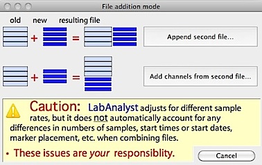
Appending is much more common than adding channels. If you select this option, the following window opens (appearance will vary depending on the number of channels and samples in the two files):
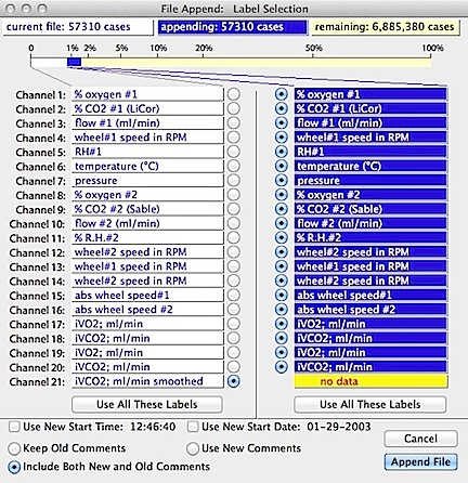
The program checks to
make sure the merged file will not exceed the current maximum file size -- unlikely unless one or both of the files are very large (a warning
is shown if this is the case). However, the program does not check to make
sure the channel contents match in the current and new files. Thus it is
possible to create a new file that contains two (or more) types of
data in a single channel (i.e., a set of temperature data from the
initial file, then gas concentration data from a second file, then
wind speed data from a third file, etc.).
Needless to say, this can cause considerable confusion unless
you are careful to avoid merging files with differing channel types.
To help avoid such mistakes, the computer provides a graphical display
of the old and new data. In this example, the file to be merged has
8 channels and the current file contains 9 channels.
LabAnalyst X will allow access to
the maximum number of channels in either the current or new file.
Sable SSCF files don't contain channel labels, so if you merge them you HAVE
to know ahead of time what the channel structure is.
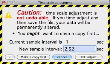
TIME SCALE ADJUSTMENT... This lets you reset the time scale, including adding or merging samples, so that two files to be merged have the same effective sample interval. This is important for timing considerations and for time-based integration functions. The window looks like this:
Back to top
Screen display basics
After a file is loaded, the 'plot area' in the top part of the screen displays
either the first channel of the file (single
channel mode) or several user-selected channels (multi-channel
mode); see the VIEW menu for details.
The screen in single-channel mode looks approximately as shown below
-- but note that immediately after loading, no block will be selected and
no data will appear in the results or block windows.
The colors of the plot
area and block window are user-selectable (VIEW)
menu and may differ from this example.
 The major components are the plot area (top half of the screen), yellow
data bar (upper left), channel indicator (upper
right), screen selection slider (bottom edge of plot area), 'toolbar'
menu buttons (across the center, just below the screen selection
slider), comments window (middle right), block window (lower
right), and analysis window (lower left). A selected block
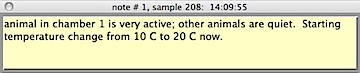
appears as a color-inverted segment of the plot area. The small 'n' buttons along the bottom of the plot area indicate notes entered while gathering data; clicking one of these buttons brings up the note text:
The major components are the plot area (top half of the screen), yellow
data bar (upper left), channel indicator (upper
right), screen selection slider (bottom edge of plot area), 'toolbar'
menu buttons (across the center, just below the screen selection
slider), comments window (middle right), block window (lower
right), and analysis window (lower left). A selected block
appears as a color-inverted segment of the plot area. The small 'n' buttons along the bottom of the plot area indicate notes entered while gathering data; clicking one of these buttons brings up the note text:
The appearance of the plot area depends on the screenwidth
(the width of the screen in pixels) and the number of cases. If the
file contains <= screenwidth cases,
data are plotted 1 pixel per case (if the number of cases is < 50% of
screenwidth, the plot is expanded,
with more than 1 pixel per case). If the total number of cases is
more than screenwidth, the X-axis will
be scaled to fit within the screen dimensions. 'Screens' (consisting
of screenwidth cases) are indicated
by vertical lines, with a crossbar at the top of the active screen.
The example shows a file containing many screenwidths
of data.
If there are more than screenwidth
cases, the bottom of the plot area will show a screen selection slider.
The currently 'active' segment of the file -- the active screen
- is indicated by the slider position. Use the slider or the left
and right arrow keys to change the active screen. To view the active
screen only (necessary for some manipulation and analysis operations), hit
the shift or return keys. Do this again to go back to
viewing the entire file (this example shows 'entire file' mode).
Any markers are shown as vertical dashed lines (this file contains
numerous markers, but they are not shown; see the VIEW
menu). While in the plot area, the cursor is a cross-hair; out of
the area it is an arrow. The data bar has a readout of case number,
elapsed time, and the value of the currently active channel at the cursor
position. The time of day is shown (24-hour scale) along the bottom of the
plot area, with optional hour indicators (vertical dotted lines).
To perform analyses and some transformations, you need to select a data
block. This can be done by the normal 'click-hold-and-drag'
method (the cursor must be within the plot area). A second method
uses individual clicks: move the cursor to the desired start point and
click once; repeat for the end point (which may be on either side
of the start point). Alternately, blocks of defined width can be selected
with single clicks (see the BLOCK
WIDTH option in the ANALYZE
menu). If there is sufficient space, you can 'shift' blocks to the left or right with the BLOCK
SHIFT commands (also in the ANALYZE
menu).
You can select blocks in 'entire file' or in 'active screen only' mode, and blocks can include multiple screens. If a single
screen is shown, mark the start with a single click, then shift
screens until the end can be marked.
A selected block is indicated as a color-inverted rectangle in the plot
area, and is scaled to fit within the block window (discrete data points
on the block window only appear if the number of included points is small).
Back to top
SAVE...
S Stores
the current file including any modifications you made. Note
that binary files saved from LabAnalyst X
have different icons than the 'raw' data files generated by LabHelper
.
SAVE
AS... Stores the current file -- or optionally
a marked block -- with any modifications you made. You may save all
channels or a subset. Files are stored in Warthog binary (file type 'WHog')
format, in Sable format (ExpeData), or as ASCII text files. The 'standard format' button saves the existing file (with any modifications
you have made with transformations, smoothing, etc.) under a new file name of your choice.
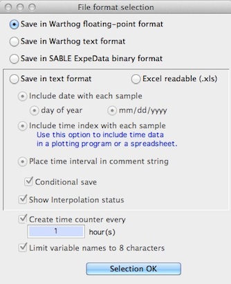
If 'standard format' was not clicked, after selecting the channels to save, the file format selection window appears, as shown below:
| If you save in Warthog text format, you retain most
all of the data that can be contained in binary files. The major exception
is in the 'comment' text. The floating-point binary format allows
very extensive comments (up to 32K of text), and the comments can include
carriage returns. When saved in Warthog text format, comments are
stripped of carriage returns (these are replaced with a single space) and
limited to a total of 252 characters. |
| As mentioned above, Sable ExpeData files do not include values for mass, flow rate, barometric pressure, temperature,
and effective volume (unless written in the comments), and comments are
limited to 240 characters. |
| The 'time counter' option creates a variable that indicates elapsed time in hours. For example, this variable would have the value of '1' for all data during the first hour, '2' for all data during the second hour, and so forth.. |
| 
|
If you select the ASCII option, you have two formatting choices:
- Timing data are stored with each case (elapsed time since acquisition began, and time of day). This option is useful
for sending files to spreadsheets or plotting programs where time data
are important.
- The sample interval and start time are stored in the comment string
(the first line in the file).
- You can also perform a 'conditional' save, which lets you save only those cases that meet a Boolean selection criterion (see below)
- NOTE: if you use conditional save, the time information (time of day, etc.) in the file will no longer be accurate. Therefore, it is highly recommended that you make backup copies of the original data before the conditional save operation.
The 'Conditional save' option lets you filter data case by case and save only the cases that meet the selection conditions. You need to specify which channel is to be tested (it is not necessary that the tested channel will be saved), one of five Boolean criteria (<, =<, =, >=, >), and a selection criterion (a number against which the individual case values in the tested channel are compared).
In this example, only cases where the value of channel 13 (wheel#1 speed in RPM) is greater than 0.5 will be saved. |
| 
|
Data files (other than ASCII) that have been saved by LabAnalyst
X have these icons:
binary files |
Warthog text files |
Sable formats |
LabAnalyst X saves some other file types, shown here (these may look different on your system, depending on what version of OS X is running):
 Preference files
|
 Script files
|
SHOW
FILE DATA Opens a window below the plot area
showing the labels of all the channels, the sample interval, the time and
date of storage, etc., and the conversions used by the LabHelper
acquisition program to change raw voltages into appropriate units (temperature,
gas concentrations, speed, etc.). The type of conversion equation
("fn") and the number of samples averaged for each recorded point
("N") are also shown.
Note that a file loaded in Sable or ASCII format may not show all of the variables.
The following example shows the file data for a 15 channel file.
Conversion equations:
Most conversion equations used by LabHelper
are 2-order polynomials (shown as "poly" in the fn column):
value = A + B*volts + C*volts2
Note that a C of zero produces
a linear conversion. Occasionally a power function is used:
value = A + B*voltsC
Note that in a power function a non-integer C will produce meaningless data if the voltage is negative;
in this condition, LabHelper sets the
results to zero. A C value
of 1 produces a linear conversion.
LabHelper allows use of the keyboard
as an event recorder, and a single channel can use a 3-degree
polynomial conversion. If data have been transformed or copied
into a new channel, no coefficients are shown.
Back to top
PRINT FILE IMAGE... Sends an image of the
file to the printer port (or a pdf file). You can usually do this by hitting the
's' key. If you have selected a block, you have the option of printing
an image of the block or of the entire file.
 Before printing, you are presented with 'Page Setup' boxes for whatever printer driver
is in use. Note that for 'US LETTER' (or similar) sized paper,
you should use landscape mode (maximum image sizes
are about 70% for portrait mode and 80% for landscape mode). If you
use other paper sizes, the recommended image sizes may be too large to fit
on the page or smaller than the available space. Before printing, you are presented with 'Page Setup' boxes for whatever printer driver
is in use. Note that for 'US LETTER' (or similar) sized paper,
you should use landscape mode (maximum image sizes
are about 70% for portrait mode and 80% for landscape mode). If you
use other paper sizes, the recommended image sizes may be too large to fit
on the page or smaller than the available space.
The printed output
will match whatever is shown in the on-screen viewing mode (Entire
File or Active Screen). A file displayed in the "Compacted
and Averaged" format will be printed in that format. If a
block has been selected, you have the option of printing only the block.
You can select which features will appear in the printout, such as labeling,
file information, comments, and markers. If the file has more than
one channel, you can print any subset of the channels.
 If you click the 'non-standard
plot heights' button, a window will open to allow customization of the
height of each printed channel: If you click the 'non-standard
plot heights' button, a window will open to allow customization of the
height of each printed channel:
The window contains a diagram of the printed page. You select the
relative height of each channel in sequence by moving the cursor on the
diagram to the desired height, and then clicking the mouse ONCE. The
channels will be redrawn one by one as their heights are selected.
Note that there is a fixed amount of room on the page, so that enlarging
one channel requires shrinking one or more of the others. Consequently,
the computer reserves an amount of space necessary for plotting the remaining
channels at the minimum possible height (and will not let you exceed that
limit). You must select plot heights for all the channels. When
done, you can accept the results, redo the plot height selection, or revert
to the normal setting (all channels plotted with equal heights).
- The speed of printing depends on the number of points and channels
to be plotted, CPU speed, the printer interface, the presence or absence
of a print spooler, and the size and selected printing resolution of the
image.
FILE
IMAGE PREVIEW... like the above routine, but it sends the image to the
screen instead of directly to the printer (you can re-route
the previewed image to the printer).
Back to top
SEND RESULTS TO
This
submenu has three items.
PRINTER
This tells LabAnalyst X
to route the data in the Results Window to the temporary printer file 'printfile'
whenever the 'P' or 'p' key is struck. Printing occurs when
you close this file with PRINT \ CLOSE FILE. After printing
the 'printfile' remains available (but it is overwritten if any additional
printing is performed).
TABULAR
FILE... Opens
a spreadsheet-format text file for storing results generated
by analysis menu operations. Data are saved in a tab-delineated format
readable by many spreadsheet programs or statistical packages. Optionally,
you can save results to an Excel-format
file (double-clickable directly into Excel).
Besides the results data, the spreadsheet file also contains column labels.
Mean, SD, N, and variable name are always saved; other parameters (start
of block, end of block, start and end time, elapsed time, analysis type,
mass, and channel number and file name) are user-selectable. You can also
enter one or two user-typed 'notes' with each case (edit fields
appear in a window over the COMMENTS window when the 'p' key is struck;
hit 'return' or click the window close button when the values are correct).
Certain analyses, such as regressions, do not fit this format and cannot
be put into tabular files.
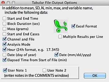
The default is one set of analysis results per line in the spreadsheet,
but if you've selected Excel
format you can use the 'Multiple results per line' option to save
the results from two to 15 different analyses per line. You need to specify
how many results you want to save initially (you can't change this when
the file is in use). Therefore, you need to keep track of the order of
analyses so as to avoid confusion later on.
If you use notes or store animal mass, these items are saved only
once per spreadsheet line (not every time you save an analysis result).
Here is a general format for one line from a file with 2 results per
line, with both user notes selected and mass saved:
Note1 · Note2
· M1 · SD1 · N1 ·
var1 · anal1
· mass ·
M2 · SD2
· N2 · var2 · anal2 <CR>
where · is a tab
character, <CR>
is a carriage return character, M1 = mean of the first result,
SD1 = SD of first result, N1 = sample size of first result,
var1 = variable for first result, anal1 = analysis for first
result, mass = body mass, M2 = mean of the second result,
etc.
Storage of results (in memory) occurs when you press the 'p' key (with
the Results window open), or select OUTPUT RESULTS. The spreadsheet
file is not saved to disk until you exit from LabAnalyst
X or use the PRINT | CLOSE FILE option.
Some additional considerations:
- Certain analyses, such as regressions and integration, do not fit this
format and cannot be put into tabular files.
- When doing waveforms or pairs-difference, pressing the 'p'
key stores BOTH frequency and amplitude data. If you want to store
one or the other, press the 'f' key to store frequency data only, or the
'a' key to store amplitude data only.
TEXT
FILE... Opens a text file for storing the contents
of the Results Window. The format of the disk file is similar to
that shown in the Results Window and is identical to the format of data
sent to the printer.
Analysis results are transferred to temporary storage in a memory table when you press the 'P' or 'p' key, or select OUTPUT RESULTS.
Real storage (writing data to disk) occurs when you select the
PRINT | CLOSE FILE ( J ) option. However, any temporary memory tables are automatically saved to disk if you quit the program.
Back to top
|